I’m currently participating in a book club for Donald Knuth’s The Art of Computer Programming. It’s run by Zartaj Majeed; you can find the details on Meetup here.

Yesterday we went over the first half of section 5.2.2, “Sorting by Exchanging.” (We’re reading in an extremely non-linear fashion.) This section starts with variations on the bubble sort. I wrote some C++ code to demonstrate three of the algorithms in this section; I figure I might as well share it.

TLDR here’s the code (Godbolt).

First of all, what’s the difference between “bubble sort” and “insertion sort” (which Knuth covers in section 5.2.1, “Sorting by Insertion”)? This StackOverflow answer really helped me with a clear answer to that. In each step of insertion sort, you’re bubbling the uppermost unsorted element through the sorted section to its proper place (Knuth calls this the “bridge-player” method). In each step of bubble sort, you’re sifting through the unsorted section to find the maximum, whose proper place is necessarily right at the bottom of the sorted section.

And in “selection sort,” you’re scanning through the unsorted section to find the maximum — doing no exchanges until the very end of the step. Only one array element moves upward in any given pass. Whereas in bubble sort, you might bubble up a few non-maximum elements before finding the actual maximum.

For me, the archetypal “bubblesort” had always been, like,

for (int i=0; i < n; ++i) {
    for (int j=0; j < n-i-1; ++j) {
        if (a[j+1] < a[j]) swap(a[j], a[j+1]);
    }
}

But Knuth presents bubblesort with a neat optimization. Think of the upward-moving elements as air bubbles bubbling through water. As the algorithm proceeds, we accumulate air at the top of our water column. In each pass, the water level will drop by at least one… but maybe more! Knuth’s archetypal bubblesort (Algorithm B in section 5.2.2) tracks the true water level in a variable called BOUND, and can terminate in fewer than n passes — as soon as BOUND hits zero, we’re done.

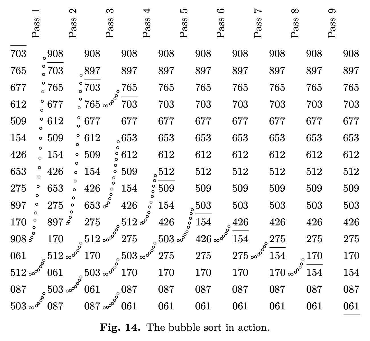
Knuth volume 3, page 106, gives the above beautiful visualization of bubblesort (complete with a little bubbly trace as each element in the watery unsorted section moves closer to the surface). The horizontal line in each column represents the water level. The trick to maintaining it is to notice that in each column, the water level is set precisely between the last two elements we exchanged in the previous step.

In Pass 4 of this example, we bubble up 512, swapping it with 426, 154, and 509. Then, since 512 was less than 612, we take up 612 as our new maximum without swapping; then 653, 677, and 703. (That is, we don’t swap any of these elements.) So the last pair of elements we swapped in Pass 4 was 509 and 512. That’s why the water level after Pass 4 has dropped five places to land between 509 and 512. We just saved four passes compared to the “naïve” nested-loop bubblesort code I presented above!

One can easily imagine a version of bubblesort with all the counters reversed, in which instead of raising up “airy” elements to the top of the column, we sink “heavy” elements to the bottom of the column. At the Meetup, Michael Zalewski referred to this variation as “rocksort.”

On pages 109–110, Knuth points out that the ordinary bubble sort has a natural tendency to sink the “rocks” toward the bottom on its own. Each time we bubble one light element upward, we’re moving it past arbitrarily many heavier elements, each of which sinks slightly downward. Notice that during Pass 4 in Figure 14, elements 061 and 087 have already reached the bottom of the column. If we were tracking a “rock level” in addition to our “water level,” we’d be able to skip comparing those two elements on every subsequent pass. Knuth writes:

This suggests the “cocktail-shaker sort,” in which alternate passes go in opposite directions.

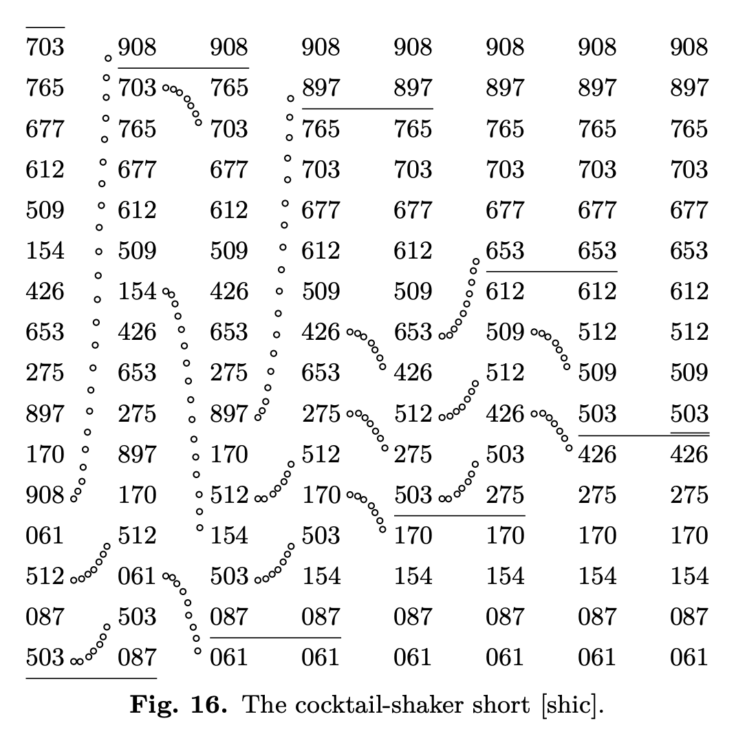
Knuth volume 3, page 110, gives the above beautiful visualization of the cocktail shaker sort. Notice that this time, alternate passes leave bubbly traces in opposite directions. The first pass bubbles air upward and lowers the water level; the second pass bubbles rocks downward and raises the rock level. After six passes, the water level meets the rock level, which means we’re done.

Finally, Knuth offers a tantalizing tidbit which took me a while to understand:

Another idea [for refining bubblesort] is to eliminate most of the exchanges; since most elements simply shift left one step during an exchange, we could achieve the same effect by viewing the array differently, shifting the origin of indexing!

What does he mean, “most elements simply shift left one step”? Well, the number of airy elements that move upward tends to be small — most of our time is spent bubbling upward the same few elements. Every element which is heavier than the current maximum ends up moving exactly one step downward (when that airy element bubbles past it). It’s true that some elements will move upward, and some elements will stay in the same place (the way Figure 14’s element 170 does, in Passes 4 through 7, before moving again in Pass 8). But a very significant majority of elements do move downward one step in each pass.

So, instead of describing an exchange as “element a[i] goes to a[i+1] and a[i+1] goes to a[i],” let’s imagine overlaying an array b such that b[0] is an alias for a[1], and let’s say “element a[i] goes to b[i+2] and a[i+1] goes to b[i+1].” Remember that a[i] probably won’t land at b[i+2] anyway, because a[i] is the current maximum and it’ll likely bubble upward by multiple places at once. Then, in the next pass, we simply change our indexing scheme so that we’re operating on the aliased array b instead of array a…

This scheme seems to cause the array to creep rightward in memory with each pass. But we can fix that by using cocktail-shaker sort instead of straight bubblesort! In the odd-numbered passes, we’ll overlay b such that b[0] is an alias for a[1] and so “sinking” elements don’t have to move. In the even-numbered passes, we’ll overlay c such that c[1] is an alias for b[0], and so “rising” elements don’t have to move. That gets our array right back to its starting position.

This refinement increases the aptness of the name “cocktail-shaker sort,” because now we’re literally shifting the whole container up and down by small increments in a repetitive motion. But paradoxically, we’re shifting the container in order to impart less motion to the elements inside; and the result is not a perfectly mixed drink but rather a perfectly unmixed one.

I decided to write up the algorithms for bubble sort, cocktail-shaker sort, and the “shifting cocktail-shaker sort” described above, to see with my own eyes the effect of Knuth’s different refinements. (Also, I needed to convince myself that the shifting shaker sort was implementable!)

Here’s my code on Godbolt (backup).

It generates an array of 100 random ints, and then sorts it in five different ways.

Naïve: 4950c 2468s - Bubble: 4931c 2468s - Shake: 3477c 2468s - Shift: 3477c 1118s - Std: 808c 70s
Naïve: 4950c 2391s - Bubble: 4814c 2391s - Shake: 3295c 2391s - Shift: 3295c  999s - Std: 820c 66s
Naïve: 4950c 2203s - Bubble: 4833c 2203s - Shake: 3007c 2203s - Shift: 3007c  913s - Std: 746c 57s
Naïve: 4950c 2652s - Bubble: 4761c 2652s - Shake: 3472c 2652s - Shift: 3472c  924s - Std: 810c 56s

Each line of output represents a different random input. 4950c means the algorithm did 4950 comparisons, and 2468s means it did 2468 swaps.

• “Naïve” is my naïve archetypal bubble sort.

• “Bubble” is Knuth’s bubble sort, tracking the water level. Notice that it does the same number of swaps as “Naïve,” but saves some comparisons because elements above the waterline needn’t be compared.

• “Shake” is Knuth’s cocktail-shaker sort, tracking both water and rock levels. Notice that it does the same number of swaps, but saves some more comparisons because elements below the seafloor needn’t be compared.

• “Shift” is my interpretation of the shifting cocktail-shaker sort. Notice that it does the same number of comparisons as “Shake,” but this time it saves some swaps. My implementation involves “pulling out” the currently bubbling element into a local variable rather than keeping it in the array; I tally a “swap” only once when the pullout is created and once when it’s put back into its final position in the array.

• “Std” is the C++ standard library’s std::sort, just for fun. I believe this is usually introsort. Notice that it does vastly fewer comparisons and vastly fewer swaps. However, be aware that the “swaps” number might be a bit of a lie; std::sort is allowed to use pullouts similar to my shifting shaker sort, and it’s not required to “report” those operations for tallying. (We could give Wrapped some special member functions to tally those operations too, but I didn’t.) Interestingly, libc++ seems to use a different and more swap-heavy algorithm for types that are move-only.

Finally, I thought it was interesting to note that all of “Naïve,” “Bubble,” and “Shake” do exactly the same number of swaps. This is because each swap exchanges two adjacent out-of-order elements, and thus decreases the array’s number of inversions by exactly 1. When the number of inversions reaches zero, the array is sorted. Therefore, every sorting algorithm that swaps only out-of-order adjacent elements must perform exactly the same number of swaps. Also, every such algorithm is stable practically by definition.

To perform fewer total swaps, you must perform some swaps that decrease the number of inversions by more than 1 at a swoop. This means you must swap some non-adjacent pairs of elements. The tradeoff is that this can easily make your sorting algorithm non-stable.

By the way, Knuth is interested in these algorithms mainly for the interesting mathematical problems that arise during analysis of their running times — not because they’re in any way efficient algorithms! If you ever have to sort a million 32-bit integers, the bubble sort would be the wrong way to go.